6 Decision Tree
References: DM Ch. 3-4, Gini index from Grokking Machine Learning
There are different ways for representing the patterns that can be discovered, and each one dictates the kind of technique that can be used to infer that output structure from data.
6.1 Output representation
6.1.1 Table
The simplest way of representing the output is to make it just the same as the input: a table. Less trivially, creating a decision or regression table might involve selecting some of the attributes, the problem is, of course, to decide which attributes select.
6.1.2 Tree
Another approach is based on the ‘divide-and-conquer’ approach to learn a tree representation, called decision tree. Nodes in a decision tree involve testing a particular attribute, leaf nodes give a classification that applies to all instances that reach the leaf, or a set of classifications, or a probability distribution. To classify a new instance, we visit the tree according to the values of the attributes tested, and classify according to the class assigned to the leaf we reach. If the tested attribute is a nominal one, the number of children is usually the number of possible values of the attribute. In this case the same attribute will not be retested further down the tree. Alternatively, values are divided in two subset, so the attribute might be tested more than once in a path according to the applied split. If the attribute is numeric, the test at a node usually determines whether its value is greater or less than a constant, giving a two-way split. If missing value is treated as an attribute value in its own, that will create a third branch. An alternative split could be based on the less than, equal to and greater than conditions. If missing values are not treated, we can simply use the most popular branch, or, a more sophisticated solution is to split the instance into pieces, send part of it down the tree and combine the decisions at the reached leaf nodes weighting the pieces.
We have many kind of decision tree:
- Regression tree: leaves of the tree are numbers that represent the average outcome for instances that reach that leaf
- Model tree: leaves are linear regression models
6.1.3 Rules
Rules are made of an antecedent (precondition), a series of tests, and a consequent (conclusion), that gives the class that apply to instances covered by that rule.
Preconditions are ANDed together, while individual rules are ORed together. However, conflicts arise when several rules with different conclusions apply.
We can create a set of rules directly off a decision tree: one rule is generated for each leaf, where the antecedent includes a condition for every node on the path from the root to that leaf. However, this procedure produces rules that are far more complex than necessary, and the problem of replicated subtree arises: decision trees cannot easily express the disjunction implied among the different rules in a set.
If a rule set gives multiple classifications for an example, one solution is to give no conclusion at all, or to count how often each rule fires on the training data and go with the most popular one.
Another problem occurs when the rules fail to classify at all. This obviously cannot happen if rules are drawn from examples, same for a decision tree, but it can happen with general rule sets. We can fail to classify that example, or choose the most frequently occurring class as a default.
A natural extension of rules is to allow them to have exceptions. Then, incremental modifications can be made to a rule set by expressing exceptions to existing rules rather than reengineering the entire set. This leads to a non-monotonic logic.
Another important consideration. Up to now, we have only considered a propositional setting, where there are no relations between attribute. Many models do not consider these relations because there is a considerable cost in doing so. One way to deal with this is to add extra attributes that account for the relation between two primary attribute. Another way is to introduce variables to express recursive rules. Sets of rules like this are called logic programs, and this area of machine learning is called inductive logic programming. Recursive definitions are hard to learn, and few practical problems require recursion.
6.1.4 Inferring rudimentary rules
This algorithm is called 1R (1-rule): it generates a one-level decision tree expressed in the form of a set of rules that all test one particular attribute.
The idea is this: we make rules that test a single attribute and branch accordingly. Each branch corresponds to a different value of the attribute. Every branch will be classified according to the most occurring class in the training data.
Each attribute generates a different set of rules, one rule for every value of the attribute.
For each attribute
    For each value of that attribute, make a rule as follows:
        count how often each class appears
        find the most frequent class
        make the rule assign that class to this attribute-value.
    Calculate the error rate of the rules.
Choose the rules with the smallest error rate
Although a very rudimentary learning scheme, 1R handles both missing values and numeric attributes:
- Missing values are treated as another attribute value
- We can convert numeric attributes into nominal ones discretizing. We can sort the training examples and place breakpoints wherever the class changes, but this produces a lot of classes and is sensible to noise. We then impose a minimum limit on the number of examples of the majority class in each partition, and merge adjacent partitions that have the same majority class.
- If a numeric attribute has missing values, an additional category is created for them, and the discretization procedure is only applied to instances with a defined value.
6.1.5 Constructing Decision Trees
First, we select an attribute to place at the root node, and make one branch for each possible value. This splits up the example set into subsets, one for every child. Now the process can be repeated recursively for each branch, using only those instances present in that node. If at any time all instances at a node have the same classification, we stop developing that part of the tree.
To choose which attribute to split one we need to have a measure of the purity of each node in order to choose the purest one. The measure of purity is called the information and is measured in bits.
We use entropy as a measure of purity entropy(p_1, \dots, p_n) = - \sum_{i = 1}^n p_i \log p_i This measure have the following (desired) properties:
- When the number of either the two classes is zero, the information is zero
- When the number of either the two classes is equal, the information reaches a maximum
- The information should allow to take a decision in several stages and not only in a single pass (So considering that we need to traverse a tree and take into account every test)
So, to choose the attribute, we compute the information gain (entropy) on the number of classes at the node (how many examples for every class we have). We then compute the average information value of these, taking into account the number of instances for each branch. Then we compute the information gain before the split. The final gain for a single attribute is given by the difference between that information gain and the average one. We choose the attribute with the maximal gain.
Ideally, the process terminates when all leaf nodes are pure. However, it might not be possible, so we stop when the data cannot be split any further, or when the information gain is zero, although it is slightly more conservative, because it is possible to encounter cases where the data can be split into subsets exhibiting identical class distributions.
Example
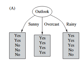
Info(Sunny) = Info([2, 3]) = - \frac{2}{5} \cdot \log_2 \frac{2}{5} - \frac{3}{5} \cdot \log_2 \frac{3}{5} = 0.971 \; \text{bits}
Info(Overcast) = Info([4, 0]) = 0 \; \text{bits}
Info(Rainy) = Info([3, 2]) = Info(Sunny) = 0.971 \; \text{bits-}
AVG = \frac{5}{14} \cdot 0.971 + \frac{4}{14} \cdot 0 + \frac{5}{14} \cdot 0.971 = 0.693 \text{ bits}
Info(Before Split) = Info([9, 5]) = -\frac{9}{14} \cdot \log_2 \frac{9}{14} - \frac{5}{14} \cdot \log_2 \frac{5}{14} = 0.940 \text{bits}
Gain(Outlook) = Info(Before Split) - AVG = 0.940 - 0.693 = 0.247 \text{ bits}
Gain(Temperature) = 0.029 bits
Gain(Humidity) = 0.152 bits
Gain(Windy) = 0.048 bits
Max(Gain) = Gain(Outlook) → we choose Outlook
The information gain tends to prefer attributes with large numbers of possible values. To compensate for this, we use a modification of the measure called the gain ratio: this is calculated by dividing the original information gain, by the intrinsic information value, that is, the information gain of the attribute:
\text{Gain Ratio} = \dfrac{\text{Gain(attribute)}}{\text{Info(attribute)}}
In some situations the gain ratio overcompensates and can lead to preferring attribute just because of a lower intrinsic information value. A fix is to choose the attribute that maximizes the gain ratio, as long as the information gain for that attribute is at least as great as the average information gain for all the attributes examined.
Example of before
Gain(Outlook) = 0.247 bits
Info(Outlook) = Info([5,4,5]) = -\frac{5}{14} \log_2 \frac{5}{14} - \frac{4}{14} \log_2 \frac{4}{14} - \frac{5}{14} \log_2 \frac{5}{14} = 1.577 \; \text{bits}
GainRatio = \frac{\text{Gain(Outlook)}}{\text{Info(Outlook)}} = \frac{0.247}{1.577} = 0.156 \text{bits}
The basic information-gain algorithm is called ID3. The one that include the gain ratio criteria as improvement, is called C4.5. Another approach is called CART, that uses Gini index instead of entropy: in a set with m elements and n classes, with a_i elements belonging to the i-th class, the Gini impurity index is
Gini = 1 - p_1^2 - p_2^2 - ... - p_n^2
where p_i = \frac{a_i}{m} . This can be interpreted as the probability that if we pick two random elements out of the set, they belong to different classes. To measure the purity of the split, we average the Gini indices of the leaves.
Gini index computes much faster than entropy because we get rid of logarithms. It is bounded to the interval (0, 0.5) while entropy is bounded in (0, 1).
Example of before
Gini(Sunny) = 1 - (\frac{2}{5})^2 - (\frac{3}{5})^2 = 0.48
Gini(Overcast) = 1 - (\frac{4}{4})^2 - 0 = 0
Gini(Rainy) = 1 - (\frac{3}{5})^2 - (\frac{2}{5})^2 = 0.48
Gini(Outlook) = \frac{0.48 + 0 + 0.48}{3} = 0.32
6.1.6 Pruning
To prevent overfitting we can prune the decision tree:
- Postpruning: take a fully-grown decision tree and discard unreliable parts. More costly but more safe
- Prepruning: early stopping, cheaper but less safe
6.1.7 Constructing Rules
We use a so-called covering approach where at each stage we identify a rule that ‘covers’ some of the instances. In contrast to decision trees and divide-and-conquer approach, the covering algorithm (separate-and-conquer) is concerned only with covering a single class, while a divide-and-conquer algorithms create a single concept description that applies to all classes.
The idea is to include as many instances of the desired class as possible and exclude as many instances of other classes as possible. That is, maximize the ratio \frac{p}{t}, with t instances and p positive examples.
One algorithm of this kind is called PRISM. It generates only correct or ‘perfect’ rules, measuring the success with the rate previously presented.
For each class C
    Initialize E to the instance set
        While E contains instances in class C
            Create a rule R with an empty left-hand side
            that predicts class C
            Until R is perfect (or there are no more attributes to use)
                do
                For each attribute A not in R, and each value v,
                    Consider A=v
                    Select A and v to maximize p/t
                    (break ties by choosing the condition
                    with the largest p)
                Add A=v to R
            Remove the instances covered by R from E
Rules produced for a particular class are not meant to be considered in order, as they all predict the same class, and no ordering is implied between the rules for one class and those for another. The disadvantage is that it’s not clear what to do when conflicting rules apply. A simple strategy to force a decision in ambiguous case is to choose the class with the most training examples or, if no classification is predicted, to choose the category with the most training examples overall. The latter case can be avoided using exceptions ensuring that any test instance receives a classification.